Air quality networks - simplifying source apportionment, supporting pollution mitigation

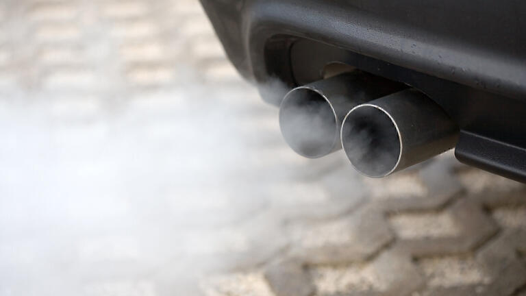
Poor urban air quality is a global problem that is worsening as the world becomes increasingly urbanised. But it is finally getting attention from the press, governments and citizens. Universities, research organisations and industry are stepping up their efforts to measure, to model and then to mitigate air pollution.

Air quality can be quantified by identifying its components, frequently divided into two broad families:
•    Inorganic gases and particles : CO, NOx (NO + NO2), SO2, O3, particulates/ aerosols: soot, ultrafine particles, PM1, PM2.5, PM10
•    Volatile Organic Compounds (VOCs): more common in indoor air, but urban air includes Polycyclic Aromatic Hydrocarbons (PAHs), benzene and other solid fuel combustion products
Inorganic gases such as carbon dioxide (CO2), methane (CH4)
and nitrous oxide (N2O) are also important because of their
effects as greenhouse gases and in the case of CO2 as a product of combustion.
If we are to monitor air quality then when we sample air quality we must first identify and quantify the polluting components. This is a difficult and frequently expensive requirement, but it is essential if we are to enable toxicologists and epidemiologists to define the health risks to our citizens. An equally important question is identification of the sources and assigning what fraction of the pollution is due to each source: this is termed source apportionment. Through source apportionment we can plan strategies to mitigate specific pollution sources through legislation, urban planning, citizen information programs, transport planning, focused academic funding and tax incentives to industry.
Historically, source apportionment has used limited data sets, usually from high quality analysis of air samples. Since the data has been sparse, various mathematical solutions have been developed. We will not discuss in detail, but two general categories are:
•    Statistical approaches which use analyses of multiple chemical species in air masses and apply statistical models to identify and apportion sources. Common computational methods include effective variance (EV), positive matrix factorization (PMF) and chemical mass balance (CMB) solutions.
•    Mechanistic computer-based models conceptually follow pollutant emissions from source to receptor. They attempt to simulate pollutants’ transport, dispersion, chemical conversion, and deposition in the atmosphere based on assumed initial map of emissions. By matching model results to measurements you can improve your emission map.
These methodologies struggle with limited data sets, but the emergence of high density air quality networks not only offers larger data sets to support the above solutions, but more usefully these networks with high spatial and temporal resolution offer a new opportunity to rethink the problem of source apportionment.
This new methodology for source apportionment relies on three major advantages of low cost air quality networks:
    dense networks with fast response to separate local and non-local sources
    source identification using network triangulation and bivariate plots with cluster analysis and simultaneous multiple pollutant parameters to profile the source.
 

Near-field or far-field source?

Dense air quality networks provide more detailed mapping of urban spaces. Coupling dense networks with fast response monitoring allows separation of local and non-local (baseline) sources. An important discovery by Cambridge is that, with fast sampling across a network, we can separate local sources (traffic, building emissions, burning, heating and cooking, and local industry) from non-local sources such as nearby cities or large industrial sites.
When one views a concentration time trace in detail, the spikes from local events are clearly seen; the slow changing background signal can be separated from the fast, local events.
Figure 2 below shows a weekly time trace of emissions from Heathrow airport.
 
Figure 2. Time traces of multiple species at Heathrow Airport (2013).
The far field background and local/ near field spikes allow us to decide if pollutants are local or long distance sources.

Polar Bivariate Plots

Adding an anemometer to measure both wind speed and wind direction allows each network node to generate a unique polar bivariate plot for each measurement, making source identification more exact and improving the reliability of source apportionment. A free website  © OpenAir! can convert node data into bivariate plots which is important for source apportionment.
Figure 3.  Bivariate plot from an air quality node near a Heathrow runway, showing pollution from aircraft and from local traffic.

Multiple Species Measurements

Local and non-local sources can be separated and by mapping the network, the plumes from non-local sources that are not throughout the network can be identified. The direction of these sources can be identified by bivariate plots. Finally, the profile of these sources can the be defined by looking at the simultaneous results for many species.
Most air quality networks monitor gases, CO2, particulates and VOCs, giving simultaneous multiple species measurements, allowing cross-measurement comparisons for more detailed source analysis.
Caption: source apportionment
Further opportunities can also be envisioned:
1    Chemical plants can establish high density networks to monitor for leaks using triangulation and knowledge of wind direction, making maintenance more targeted.
2    Citizen scientists can build their own ad-hoc networks and learn about air quality in their neighbourhood; in fact, air quality boards that plug into Raspberry Pi’s are commercially available.
3     Although the discussion is with fixed site networks, mobile/ portable air quality monitors with GPS can rapidly identify sources and give limited apportion information

What next?

•    Reducing pollution starts with finding the sources and identifying the polluting species: source apportionment.
•    While previous methods have used advanced modelling with a minimum of data, air quality networks provide very large data sets, improving our models.
•    Separating the local and non-local sources and then using polar bivariate plots allows us to identify the location of the sources- both direction and distance.
•    Profiling the polluting source using simultaneous data from many sensors allows us identify the species, directing the actions to mitigate the polluting source.